The mean tells you the centre — the standard deviation tells you the spread
Two classes can both average 70 on a test while being nothing alike: in one, everyone scores between 65 and 75; in the other, half the class scores 40 and half scores 100. The standard deviation (SD) is the number that separates those two stories. It measures the typical distance between each value and the mean, in the same units as the data itself — marks, dollars, kilograms. A small SD means the values huddle near the mean; a large SD means they are scattered. This calculator takes any list of numbers and returns the mean, both variances and both standard deviations, and — the part most calculators hide — a step table showing every value's deviation from the mean and its square, so you can watch the total being built and check it yourself. If you only need the centre, our average calculator covers mean, median and mode; this page exists for the spread.
The formula, step by step
Step 1 — mean: x̄ = (sum of all values) ÷ NStep 2 — deviations: subtract the mean from every value, then square each resultStep 3 — variance: population σ² = (sum of squared deviations) ÷ N · sample s² = (sum of squared deviations) ÷ (N − 1)Step 4 — standard deviation: σ = √σ² · s = √s² (undo the squaring with a square root)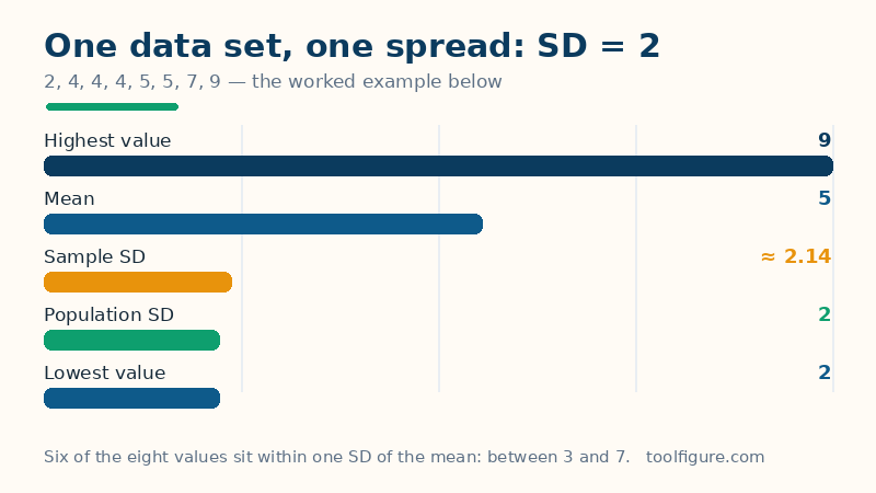
Every symbol, in plain words. N is how many values you have. x̄ (read "x-bar") is the mean — the balancing point of the data. A deviation is one value's signed distance from that mean; the deviations always add to exactly zero, which is useless as a spread measure, so step 2 squares them — squaring kills the signs and punishes far-off values more than near ones. The average of those squares is the variance, and step 4 takes its square root to bring the units back from "marks squared" to plain marks: that root is the standard deviation. The only fork in the road is step 3's divisor. Divide by N when your list is the entire group you care about (population). Divide by N − 1 when your list is a sample standing in for a bigger group (sample) — the smaller divisor inflates the answer slightly, honestly compensating for the fact that a sample tends to hug its own mean a little closer than it hugs the true population mean. That adjustment is called Bessel's correction.
Worked example: 2, 4, 4, 4, 5, 5, 7, 9
This eight-number set is the classic teaching example, and every figure below is printed by the calculator above. Step 1: the sum is 2 + 4 + 4 + 4 + 5 + 5 + 7 + 9 = 40, so the mean is 40 ÷ 8 = 5. Step 2: the deviations from 5 are −3, −1, −1, −1, 0, 0, 2 and 4; squared, they are 9, 1, 1, 1, 0, 0, 4 and 16. Step 3: those squares add to 9 + 1 + 1 + 1 + 0 + 0 + 4 + 16 = 32. As a population, the variance is 32 ÷ 8 = 4; as a sample it is 32 ÷ 7 ≈ 4.5714. Step 4: the population standard deviation is √4 = 2 exactly, and the sample standard deviation is √4.5714 ≈ 2.1381. Read the answer back in plain language: the values centre on 5, and a typical value sits about 2 away from 5. Reality check: the interval from one SD below the mean to one above (3 to 7) holds 6 of the 8 values — most of them, as it should. The bars below draw the same example: the centre at 5, the spread of 2 around it, and the full 2-to-9 range it summarises.
A second verified example — and the population-versus-sample gap
| Data set | Mean | Squared devs sum | Population SD | Sample SD |
|---|---|---|---|---|
| 2, 4, 4, 4, 5, 5, 7, 9 | 5 | 32 | 2 | 2.1381 |
| 10, 12, 23, 23, 16, 23, 21, 16 | 18 | 192 | 4.899 | 5.2372 |
| 1, 2, 3, 4, 5 | 3 | 10 | 1.4142 | 1.5811 |
The second row, checked by hand: the values sum to 144, the mean is 18, the deviations are −8, −6, 5, 5, −2, 5, 3, −2, their squares are 64, 36, 25, 25, 4, 25, 9, 4, and those squares total 192 — giving a population variance of 192 ÷ 8 = 24 and an SD of √24 ≈ 4.899, against a sample variance of 192 ÷ 7 ≈ 27.4286 and an SD of ≈ 5.2372. Two lessons live in this table. First, the sample SD is always the larger of the pair (same numerator, smaller divisor), and the gap shrinks as N grows — at N = 5 the sample figure is 12% higher, at N = 8 about 7% higher. Second, spread is about the data, not the centre: the tidy 1-to-5 ladder has a smaller SD than either real-world set, even though all three means are ordinary numbers. Comparing spreads like this is also how grade distributions get read in practice — the same machinery that sits behind a class's GPA spread in our GPA calculator.
Reading a standard deviation without fooling yourself
Three habits keep SD honest. First, SD is not the average distance from the mean — that simpler idea exists (the mean absolute deviation) and is always a bit smaller, because squaring over-weights the far values; SD is a root-mean-square distance, and for roughly bell-shaped data it buys you the famous rule of thumb: about 68% of values within one SD of the mean, 95% within two, 99.7% within three. Our worked example fits it loosely (6 of 8 inside one SD) because eight points are too few to be smooth — the rule describes large, bell-shaped sets, not every list. Second, an SD of 0 is a real answer: it means every value is identical, not that something broke. Third, outliers move SD a lot, precisely because their deviations get squared: change the 9 in the worked example to 90 and the population SD leaps from 2 to about 29, while the median barely stirs. When a data set has wild outliers, report the median alongside the SD, and treat any single spread number with suspicion — the same caution this site applies to averages generally.
Frequently asked questions
What is the difference between population and sample standard deviation?
The divisor. Population SD divides the sum of squared deviations by N — use it when your list is the entire group you care about. Sample SD divides by N − 1 (Bessel's correction) — use it when your list is a sample from a larger group, because a sample hugs its own mean slightly closer than the true population mean. For 2, 4, 4, 4, 5, 5, 7, 9 the answers are 2 (population) and about 2.1381 (sample).
Why are the deviations squared — why not just average the distances?
Two reasons. Raw deviations always sum to exactly zero (the values above the mean cancel those below), so they must be made positive first — and squaring, unlike absolute value, also penalises one far-off value more than several near ones, which matches how spread actually feels. The square root at the end restores the original units, turning 'marks squared' back into marks.
Can the standard deviation be zero or negative?
Zero, yes — it means every value in the list is identical, so there is no spread at all. Negative, never: the SD is a square root of an average of squares, and squares are never negative. If a calculation ever shows you a negative standard deviation, the calculation — not your data — is broken.
What is a 'good' or normal standard deviation?
There is no universal good value, because SD carries the units of your data: an SD of 2 marks on a test marked out of 10 is wide, while 2 marks out of 100 is tight. Judge it against the mean and the scale: as a rough feel, an SD under about 10% of the mean means tightly clustered data, and over 30% means widely scattered. The 68-95-99.7 rule then tells you where most values should fall.
How many numbers can I paste in, and how are they read?
Up to 1,000 numbers, separated by commas — pasting straight from a spreadsheet column works if you replace the line breaks with commas, or copy a comma-separated row. Decimals are fine, negative numbers are fine, and the step table shows the first 50 squared deviations while the totals always use every value you entered.